8 Per-SNP QC
Now that we removed samples, we can focus on low-quality variants.
8.1 SNP call rates
We start by calculating the missing genotype rate for each SNP, in other words the per-SNP call rate.
plink --bfile dummy_project/clean_inds_data --missing --out dummy_project/clean_inds_dataLet’s visualize the results to identify a threshold for extreme genotype failure rate. We chose a callrate threshold of 3%, but it’s arbitrary and depending on the dataset, the data (visualization), and the number of samples (Figure 8.1).
library("data.table")
clean_LMISS <- data.table::fread("dummy_project/clean_inds_data.lmiss")

clean_LMISS$callrate <- 1 - clean_LMISS$F_MISSlibrary("ggpubr")
clean_LMISS_plot <- ggpubr::gghistogram(clean_LMISS, x = "callrate",
add = "mean", add.params = list(color = "#595A5C", linetype = "dashed", size = 1),
rug = TRUE, bins = 50,
color = "#1290D9", fill = "#1290D9",
xlab = "per SNP call rate") +
ggplot2::geom_vline(xintercept = 0.95, linetype = "dashed",
color = "#E55738", size = 1)
ggplot2::ggsave("dummy_project/gwas-qc-snp-call-rate.png", plot = clean_LMISS_plot)
clean_LMISS_plot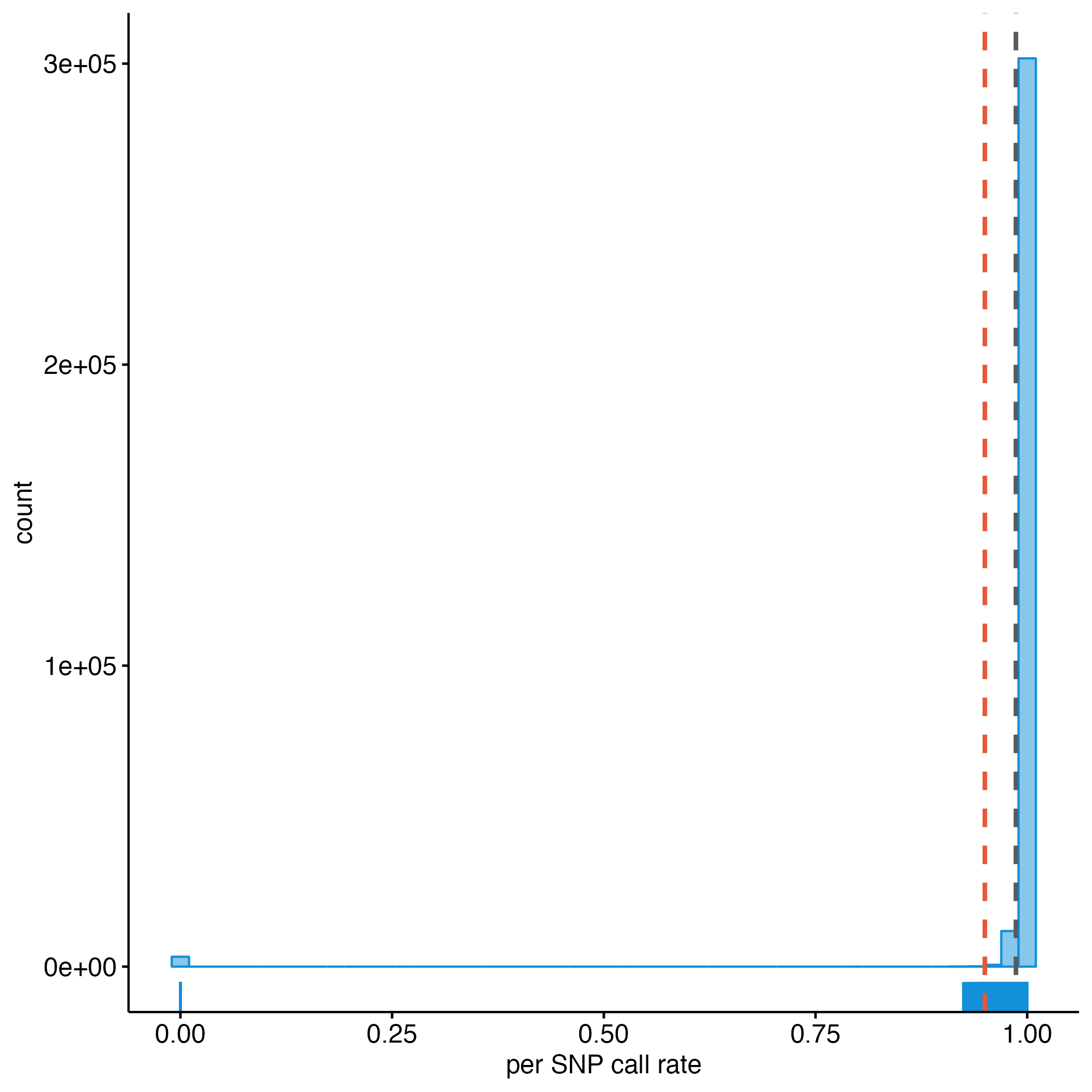
Figure 8.1: Per SNP call rate.
8.2 Differential SNP call rates
There could also be differences in genotype call rates between cases and controls. It is very important to check for this because these differences could lead to spurious associations. We can test all markers for differences in call rate between cases and controls, or based on other criteria.
plink --bfile dummy_project/clean_inds_data --test-missing --out dummy_project/clean_inds_dataLet’s collect all the SNPs with a significantly different (P < 0.00001) missing data rate between cases and controls.
cat dummy_project/clean_inds_data.missing | awk '$5 < 0.00001' | awk '{ print $2 }' > dummy_project/fail-diffmiss-qc.txt8.3 Allele frequencies
We should also get an idea on what the allele frequencies are in our dataset. Low frequent SNPs should probably be excluded, as these are uninformative when monomorphic (allele frequency = 0), or they may lead to spurious associations.
plink --bfile dummy_project/clean_inds_data --freq --out dummy_project/clean_inds_dataLet’s also plot these data. You can view the result below, and try it yourself (Figure 8.2).
clean_FREQ_plot <- ggpubr::gghistogram(clean_FREQ, x = "MAF",
                                       add = "mean", add.params = list(color = "#595A5C", linetype = "dashed", size = 1),
                                       rug = TRUE,
                                       color = "#1290D9", fill = "#1290D9",
                                       xlab = "minor allele frequency") +
  ggplot2::geom_vline(xintercept = 0.05, linetype = "dashed",
                      color = "#E55738", size = 1)

ggplot2::ggsave("dummy_project/gwas-qc-snp-freq.png", plot = clean_FREQ_plot)
clean_FREQ_plot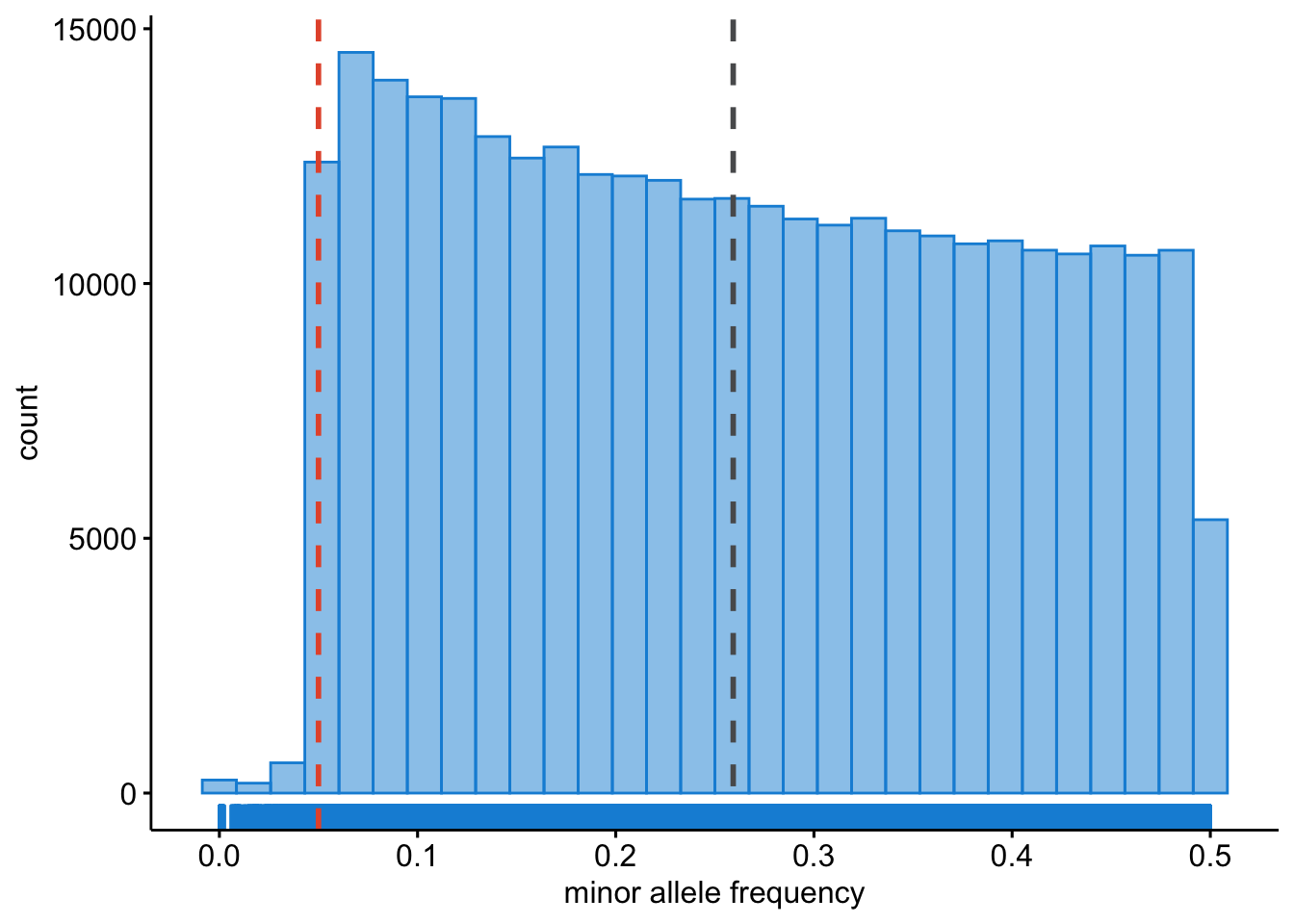
Figure 8.2: Minor allele frequency.
8.3.1 A note on allele coding
Oh, one more thing about alleles.
PLINK codes alleles as follows:
A1 = minor allele, the least frequent allele A2 = major allele, the most frequent allele
And when you use PLINK the flag --freq or --maf is always relative to the A1-allele, as is the odds ratio (OR) or effect size (beta).
However, SNPTEST makes use of the so-called OXFORD-format, this codes alleles as follows:
A = the ‘other’ allele B = the ‘coded’ allele
When you use SNPTEST it will report the allele frequency as CAF, in other words the coded allele frequency, and the effect size (beta) is always relative to the B-allele. This means, CAF could be the MAF, or minor allele frequency, but this is not a given.
In other words, always make sure what the allele-coding of a given program, be it PLINK, SNPTEST, GCTA, et cetera, is! I cannot stress this enough. Ask yourself: ‘what is the allele frequency referring to?’, ‘the effect size is relative to…?’.
Right, let’s continue.
8.4 Hardy-Weinberg Equilibrium
Because we are performing a case-control genome-wide association study, we probably expect some differences in Hardy-Weinberg Equilibrium (HWE), but extreme deviations are probably indicative of genotyping errors.
plink --bfile dummy_project/clean_inds_data --hardy --out dummy_project/clean_inds_dataLet’s also plot these data. You can view the result below, and type over the code to do it yourself.
clean_HWE <- data.table::fread("dummy_project/clean_inds_data.hwe")
clean_HWE$logP <- -log10(clean_HWE$P)
clean_HWE_plot <- ggpubr::gghistogram(clean_HWE, x = "logP",
add = "mean",
add.params = list(color = "#595A5C", linetype = "dashed", size = 1),
rug = TRUE,
# color = "#1290D9", fill = "#1290D9",
color = "TEST", fill = "TEST",
palette = "lancet",
facet.by = "TEST",
bins = 50,
xlab = "HWE -log10(P)") +
ggplot2::geom_vline(xintercept = 5, linetype = "dashed",
color = "#E55738", size = 1)
ggplot2::ggsave("dummy_project/gwas-qc-snp-hwe.png", plot = clean_HWE_plot)
clean_HWE_plot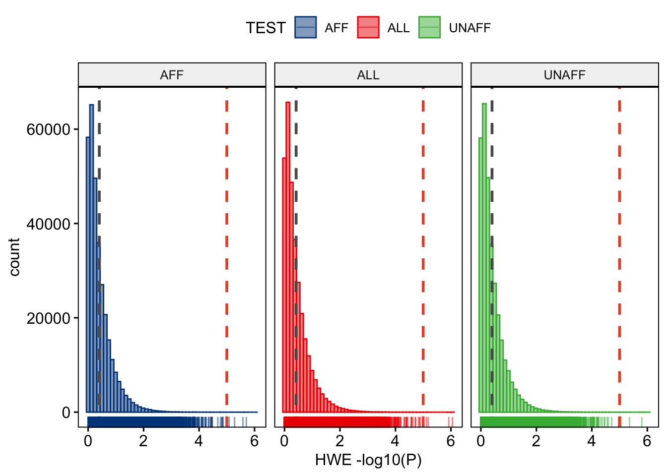
Figure 8.3: Hardy-Weinberg Equilibrium p-values per stratum.
8.5 Final SNP QC
We are ready to perform the final QC. After inspecting the graphs we will filter on a MAF < 0.01, call rate < 0.05, and HWE < 0.00001 (Figure 8.3), in addition those SNPs that failed the differential call rate test will be removed.
plink --bfile dummy_project/clean_inds_data --exclude dummy_project/fail-diffmiss-qc.txt --maf 0.01 --geno 0.05 --hwe 0.00001 --make-bed --out dummy_project/cleandata8.6 A Milestone
Congratulations. You reached a very important milestone. Now that you filtered samples and SNPs, we can finally start the association analyses in Chapter 9.