13 WTCCC1: quality control
As usual, we start by exploring the data in hand.
First, let’s make a clean slate and create a working directory for the WTCCC1 data.
clear
mkdir -v ~/wtccc1
Next, we’ll run a few plink commands
plink --bfile ~/data/shared/wtccc1/CADn1871_500Kb37fwd --bmerge ~/data/shared/wtccc1/UKBSn1397_500Kb37fwd --make-bed --out wtccc1/wtccc1 && \
plink --bfile wtccc1/wtccc1 --freq --out wtccc1/wtccc1 && \
plink --bfile wtccc1/wtccc1 --hardy --out wtccc1/wtccc1 && \
plink --bfile wtccc1/wtccc1 --missing --out wtccc1/wtccc1 && \
plink --bfile wtccc1/wtccc1 --test-missing --out wtccc1/wtccc1

cat wtccc1/wtccc1.missing | awk '$5 < 0.00001' | awk '{ print $2 }' > wtccc1/wtccc1-fail-diffmiss-qc.txtlibrary("data.table")
wtccc1_HWE <- data.table::fread("wtccc1/wtccc1.hwe")
wtccc1_FRQ <- data.table::fread("wtccc1/wtccc1.frq")
wtccc1_IMISS <- data.table::fread("wtccc1/wtccc1.imiss")
wtccc1_LMISS <- data.table::fread("wtccc1/wtccc1.lmiss")
wtccc1_HWE$logP <- -log10(wtccc1_HWE$P)
wtccc1_LMISS$callrate <- 1 - wtccc1_LMISS$F_MISS
wtccc1_IMISS$callrate <- 1 - wtccc1_IMISS$F_MISSLet’s investigate the HWE p-value in the whole cohort, and per stratum (cases and controls) with the code below.
library("ggpubr")

ggpubr::gghistogram(wtccc1_HWE, x = "logP",
                    add = "mean",
                    add.params = list(color = "#595A5C", linetype = "dashed", size = 1),
                    rug = TRUE,
                    # color = "#1290D9", fill = "#1290D9",
                    color = "TEST", fill = "TEST",
                    palette = "lancet",
                    facet.by = "TEST",
                    bins = 50,
                    xlab = "HWE -log10(P)") +
  ggplot2::geom_vline(xintercept = 5, linetype = "dashed",
                      color = "#E55738", size = 1)
ggplot2::ggsave("wtccc1/wtccc1-hwe.png", plot = last_plot())
This will result in Figure 13.1.
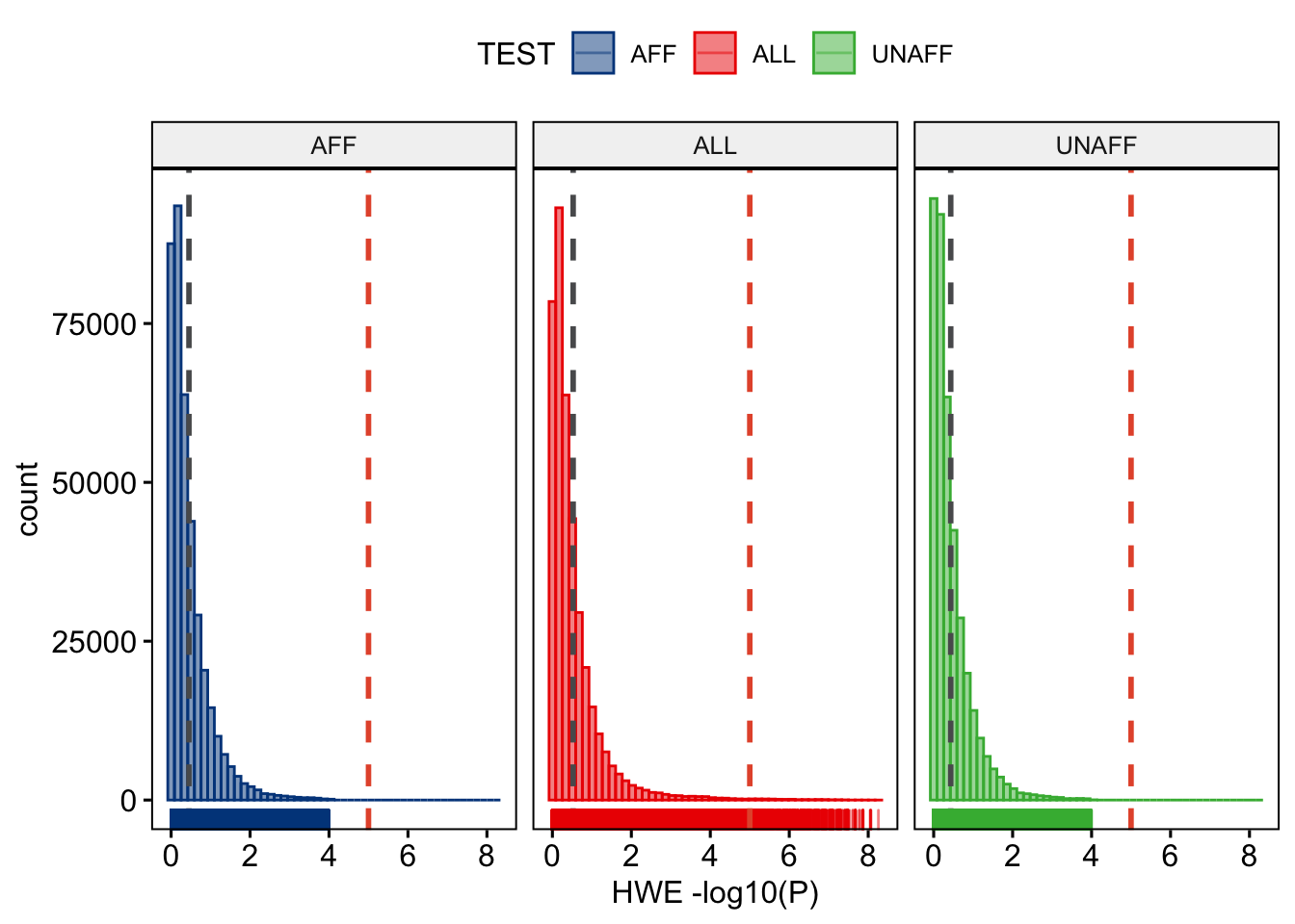
Figure 13.1: Stratified HWE p-values.
We should also inspect the allele frequencies. Note that by default PLINK (whether v0.7, v1.9, or v2.0) stores the alleles as minor (A1) and major (A2), and therefore --maf always calculates the frequency of the minor allele (A1).
ggpubr::gghistogram(wtccc1_FRQ, x = "MAF",
                    add = "mean", add.params = list(color = "#595A5C", linetype = "dashed", size = 1),
                    rug = TRUE,
                    color = "#1290D9", fill = "#1290D9",
                    xlab = "minor allele frequency") +
  ggplot2::geom_vline(xintercept = 0.05, linetype = "dashed",
                      color = "#E55738", size = 1)
ggplot2::ggsave("wtccc1/wtccc1-freq.png", plot = last_plot())
This will result in Figure 13.2.
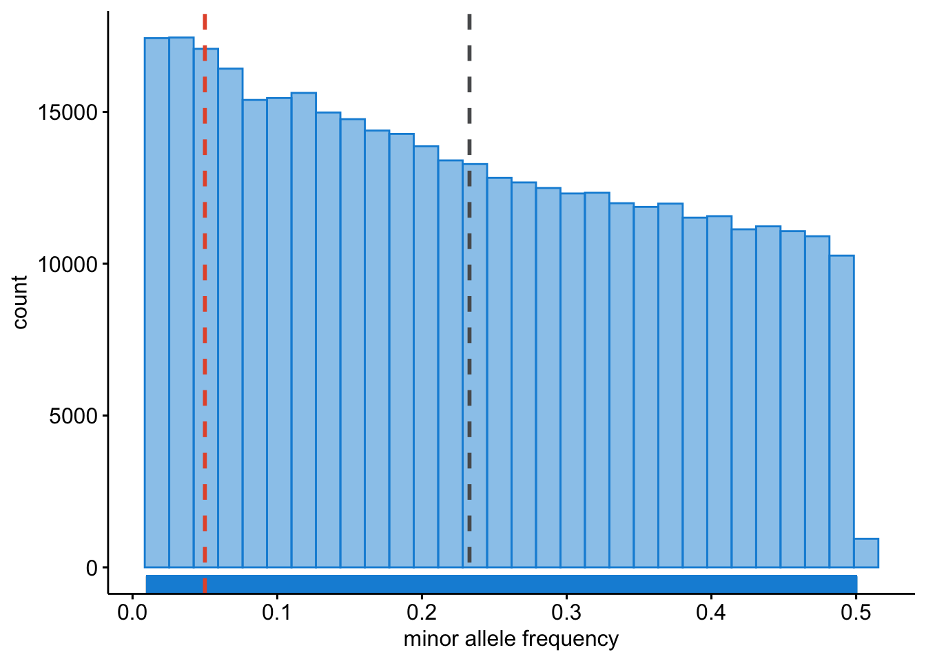
Figure 13.2: Minor allele frequencies.
There could be sample with very poor overall call rate, where for many SNPs there is no data. We will want to identify these samples and exclude them.
ggpubr::gghistogram(wtccc1_IMISS, x = "callrate",
                    add = "mean", add.params = list(color = "#595A5C", linetype = "dashed", size = 1),
                    rug = TRUE, bins = 50,
                    color = "#1290D9", fill = "#1290D9",
                    xlab = "per sample call rate") +
  ggplot2::geom_vline(xintercept = 0.95, linetype = "dashed",
                      color = "#E55738", size = 1)
ggplot2::ggsave("wtccc1/wtccc1-sample-call-rate.png", plot = last_plot())
This will result in Figure 13.3.
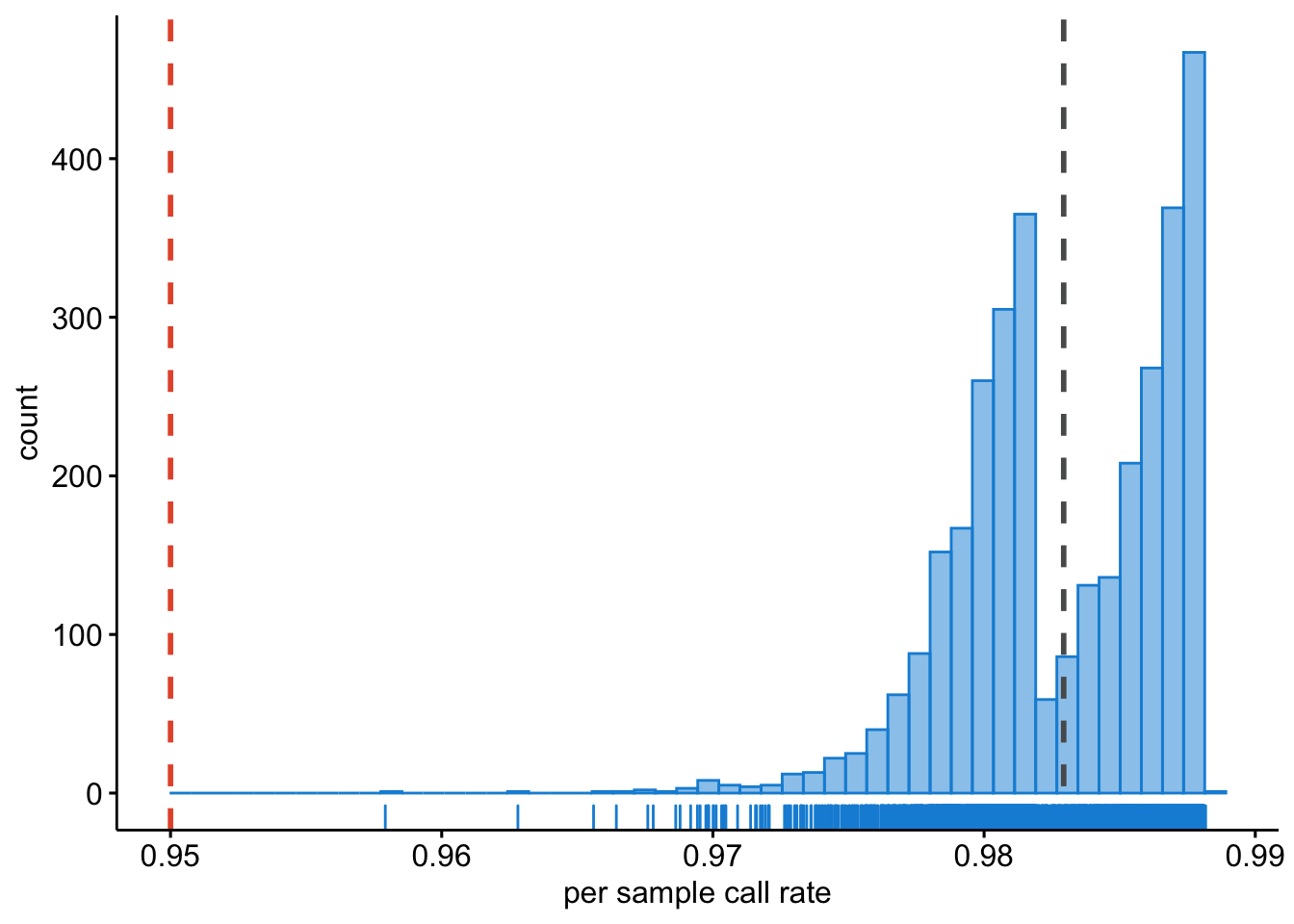
Figure 13.3: Per sample call rate.
Question: What do you notice in the ‘per sample call rate’ graph? Can you think of a reason why this is? And how would you deal with this?
Lastly, we must inspect the per SNP call rate; we need to know if there are SNPs that have no data for many samples. We will want to identify such SNPs and exclude these.
ggpubr::gghistogram(wtccc1_LMISS, x = "callrate",
                    add = "mean", add.params = list(color = "#595A5C", linetype = "dashed", size = 1),
                    rug = TRUE, bins = 50,
                    color = "#1290D9", fill = "#1290D9",
                    xlab = "per SNP call rate") +
  ggplot2::geom_vline(xintercept = 0.95, linetype = "dashed",
                      color = "#E55738", size = 1)
ggplot2::ggsave("wtccc1/wtccc1-hwe.png", plot = last_plot())
This will result in Figure 13.4.
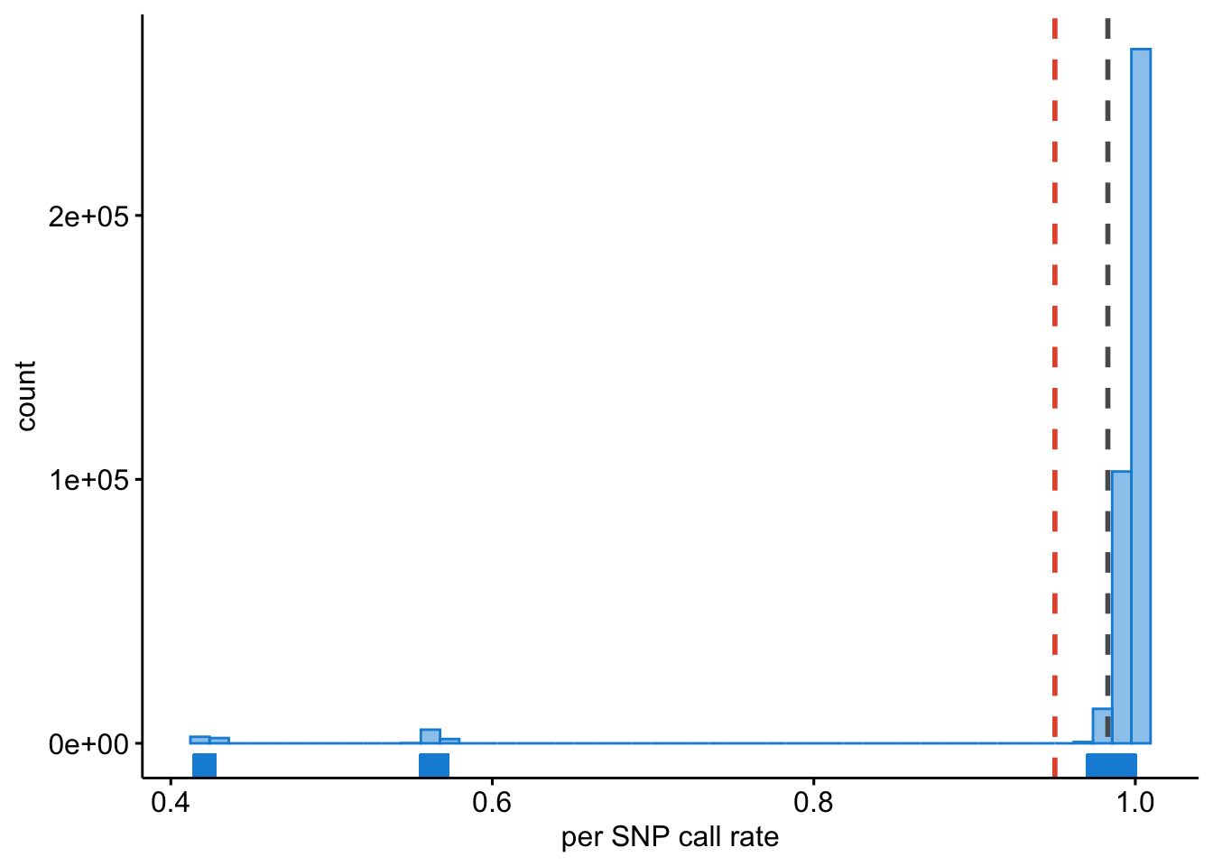
Figure 13.4: Per SNP call rate.
13.1 Quality control
Now that we have handle on the data, we can filter it.
plink --bfile wtccc1/wtccc1 --exclude wtccc1/wtccc1-fail-diffmiss-qc.txt --maf 0.01 --geno 0.05 --hwe 0.00001 --make-bed --out wtccc1/wtccc1_cleanQuestion: Do you have any thoughts on that? Do you agree with the filters I set below? How would you do it differently and why?
13.2 Ancestral background
If these individuals are all from the United Kingdom, we are certain there will be admixture from other populations given UK’s history. Let’s project the WTCCC1 data on 1000G phase 1 populations.
We will face the same issue as before with our dummy dataset with respect to EIGENSOFT. So I created the data for you to skip to the Plotting PCA section immediately. Regardless, in the Preparing PCA and Running PCA sections I show you how to get there.
13.2.1 Preparing PCA
Filtering WTCCC1
For PCA we need to perform extreme clean.
plink --bfile wtccc1/wtccc1_clean --maf 0.1 --geno 0.1 --indep-pairwise 100 50 0.2 --exclude ~/data/shared/support/exclude_problematic_range.txt --make-bed --out wtccc1/wtccc1_temp

plink --bfile wtccc1/wtccc1_temp --exclude wtccc1/wtccc1_temp.prune.out --make-bed --out wtccc1/wtccc1_extrclean

rm -fv wtccc1/wtccc1_temp*

cat wtccc1/wtccc1_extrclean.bim | awk '{ print $2 }' > wtccc1/wtccc1_extrclean.variants.txt

cat wtccc1/wtccc1.bim | grep "rs" > wtccc1/all.variants.txt
Notice that you are using real world data: there are thousands of variants ‘pruned’ due to the --indep-pairwise 100 50 0.2-flag.
Merging WTCCC1 with 1000G phase 1
Now we are ready to extract the WTCCC1 variants from the 1000G phase 1 reference
plink --bfile ~/data/shared/ref_1kg_phase1_all/1kg_phase1_all --extract wtccc1/all.variants.txt --make-bed --out wtccc1/1kg_phase1_wtccc1Extracting the A/T and C/G SNPs as well.
cat wtccc1/1kg_phase1_wtccc1.bim | \
awk '($5 == "A" && $6 == "T") || ($5 == "T" && $6 == "A") || ($5 == "C" && $6 == "G") || ($5 == "G" && $6 == "C")' | awk '{ print $2, $1, $4, $3, $5, $6 }' \
> wtccc1/all.1kg_wtccc1.atcg.variants.txt
plink --bfile wtccc1/1kg_phase1_wtccc1 --exclude wtccc1/all.1kg_wtccc1.atcg.variants.txt --make-bed --out wtccc1/1kg_phase1_wtccc1_no_atcg
plink --bfile wtccc1/1kg_phase1_wtccc1_no_atcg --extract wtccc1/wtccc1_extrclean.variants.txt --make-bed --out wtccc1/1kg_phase1_raw_no_atcg_wtccc1Finally we will merge the datasets.
plink --bfile wtccc1/wtccc1_extrclean --bmerge wtccc1/1kg_phase1_raw_no_atcg_wtccc1 --maf 0.1 --geno 0.1 --exclude ~/data/shared/support/exclude_problematic_range.txt --make-bed --out wtccc1/wtccc1_extrclean_1kg13.2.2 Running PCA
Great, we’ve prepared our dummy project data and merged this with 1000G phase 1. Let’s execute the PCA using --pca in PLINK.
plink --bfile wtccc1/wtccc1_extrclean_1kg --pca --out wtccc1/wtccc1_extrclean_1kg13.2.3 Plotting PCA
If all is peachy, you were able to run the PCA for the WTCCC1 data against 1000G phase 1. Using --pca in plink we have calculated principal components (PCs) and we can now start plotting them. Let’s create a scatter diagram of the first two principal components just like we did with the dummy data.
And we should visualize the PCA results: are these individuals really all from European (UK) ancestry?
PCA_eigenval <- data.table::fread("wtccc1/wtccc1_extrclean_1kg.eigenval")
PCA_eigenvec <- data.table::fread("wtccc1/wtccc1_extrclean_1kg.eigenvec")
ref_pop_raw <- data.table::fread("~/data/shared/ref_1kg_phase1_all/1kg_phase1_all.pheno")
wtccc1_pop <- data.table::fread("wtccc1/wtccc1.fam")
# Rename some
names(PCA_eigenval)[names(PCA_eigenval) == "V1"] <- "Eigenvalue"
names(PCA_eigenvec)[names(PCA_eigenvec) == "V1"] <- "FID"
names(PCA_eigenvec)[names(PCA_eigenvec) == "V2"] <- "IID"
names(PCA_eigenvec)[names(PCA_eigenvec) == "V3"] <- "PC1"
names(PCA_eigenvec)[names(PCA_eigenvec) == "V4"] <- "PC2"
names(PCA_eigenvec)[names(PCA_eigenvec) == "V5"] <- "PC3"
names(PCA_eigenvec)[names(PCA_eigenvec) == "V6"] <- "PC4"
names(PCA_eigenvec)[names(PCA_eigenvec) == "V7"] <- "PC5"
names(PCA_eigenvec)[names(PCA_eigenvec) == "V8"] <- "PC6"
names(PCA_eigenvec)[names(PCA_eigenvec) == "V9"] <- "PC7"
names(PCA_eigenvec)[names(PCA_eigenvec) == "V10"] <- "PC8"
names(PCA_eigenvec)[names(PCA_eigenvec) == "V11"] <- "PC9"
names(PCA_eigenvec)[names(PCA_eigenvec) == "V12"] <- "PC10"
names(PCA_eigenvec)[names(PCA_eigenvec) == "V13"] <- "PC11"
names(PCA_eigenvec)[names(PCA_eigenvec) == "V14"] <- "PC12"
names(PCA_eigenvec)[names(PCA_eigenvec) == "V15"] <- "PC13"
names(PCA_eigenvec)[names(PCA_eigenvec) == "V16"] <- "PC14"
names(PCA_eigenvec)[names(PCA_eigenvec) == "V17"] <- "PC15"
names(PCA_eigenvec)[names(PCA_eigenvec) == "V18"] <- "PC16"
names(PCA_eigenvec)[names(PCA_eigenvec) == "V19"] <- "PC17"
names(PCA_eigenvec)[names(PCA_eigenvec) == "V20"] <- "PC18"
names(PCA_eigenvec)[names(PCA_eigenvec) == "V21"] <- "PC19"
names(PCA_eigenvec)[names(PCA_eigenvec) == "V22"] <- "PC20"
names(wtccc1_pop)[names(wtccc1_pop) == "V1"] <- "Family_ID"
names(wtccc1_pop)[names(wtccc1_pop) == "V2"] <- "Individual_ID"
names(wtccc1_pop)[names(wtccc1_pop) == "V5"] <- "Gender"
names(wtccc1_pop)[names(wtccc1_pop) == "V6"] <- "Phenotype"
wtccc1_pop$V3<- NULL
wtccc1_pop$V4<- NULL
wtccc1_pop$Population <- wtccc1_pop$Phenotype
wtccc1_pop$Population[wtccc1_pop$Population == 2] <- "Case"
wtccc1_pop$Population[wtccc1_pop$Population == 1] <- "Control"# we subset the data we need
ref_pop <- subset(ref_pop_raw, select = c("Family_ID", "Individual_ID", "Gender", "Phenotype", "Population"))
rm(ref_pop_raw)
# we combine the reference and dummy information
ref_wtccc1_pop <- rbind(wtccc1_pop, ref_pop)PCA_1kG <- merge(PCA_eigenvec,
ref_wtccc1_pop,
by.x = "IID",
by.y = "Individual_ID",
sort = FALSE,
all.x = TRUE)# Population Description Super population Code Counts
# ASW African Ancestry in Southwest US AFR 4 #49A01D
# CEU Utah residents with Northern and Western European ancestry EUR 7 #E55738
# CHB Han Chinese in Bejing, China EAS 8 #9A3480
# CHS Southern Han Chinese, China EAS 9 #705296
# CLM Colombian in Medellin, Colombia MR 10 #8D5B9A
# FIN Finnish in Finland EUR 12 #2F8BC9
# GBR British in England and Scotland EUR 13 #1290D9
# IBS Iberian populations in Spain EUR 16 #1396D8
# JPT Japanese in Tokyo, Japan EAS 18 #D5267B
# LWK Luhya in Webuye, Kenya AFR 20 #78B113
# MXL Mexican Ancestry in Los Angeles, California AMR 22 #F59D10
# PUR Puerto Rican in Puerto Rico AMR 25 #FBB820
# TSI Toscani in Italy EUR 27 #4C81BF
# YRI Yoruba in Ibadan, Nigeria AFR 28 #C5D220
PCA_1kGplot <- ggpubr::ggscatter(PCA_1kG,
x = "PC1",
y = "PC2",
color = "Population",
palette = c("#49A01D",
"#595A5C",
"#E55738",
"#9A3480",
"#705296",
"#8D5B9A",
"#A2A3A4",
"#2F8BC9",
"#1290D9",
"#1396D8",
"#D5267B",
"#78B113",
"#F59D10",
"#FBB820",
"#4C81BF",
"#C5D220"),
xlab = "principal component 1", ylab = "principal component 2") +
ggplot2::geom_vline(xintercept = 0.0023, linetype = "dashed",
color = "#E55738", size = 1)
p2 <- ggpubr::ggpar(PCA_1kGplot,
title = "Principal Component Analysis",
subtitle = "Reference population: 1000 G, phase 1",
legend.title = "Populations", legend = "right")
ggplot2::ggsave("wtccc1/wtccc1-qc-pca-1000g.png", plot = p2)
p2
rm(p2)We expect most individuals from the WTCCC to be 100% British, but a substantial group will have a different ancestral background as shown in the Figure 13.5 you just made.
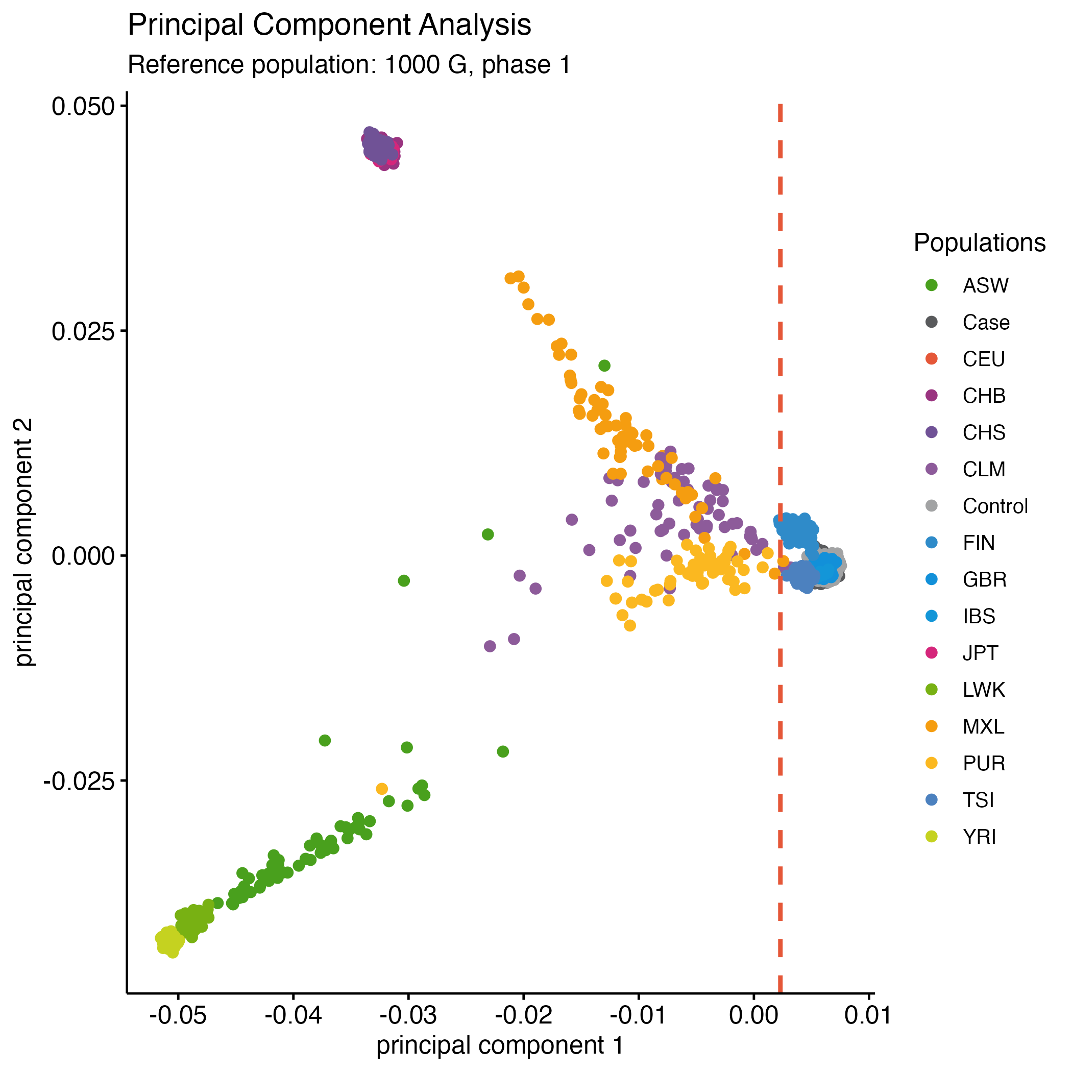
Figure 13.5: PCA - WTCCC1 vs. 1000G
13.2.4 Removing samples
In a similar fashion as in the example gwas and rawdata datasets, you should consider to remove the samples below the threshold based on this PCA (Figure 13.5).
Go ahead, try that.
You’re code would be something like below:
cat wtccc1/wtccc1_extrclean_1kg.eigenvec | \
awk '$3 < 0.0023' | awk '{ print $1, $2 }' > wtccc1/fail-ancestry-QC.txt
Next we filter these samples and get a final fully QC’d dataset.
plink --bfile wtccc1/wtccc1_clean --exclude wtccc1/fail-ancestry-QC.txt --make-bed --out wtccc1/wtccc1_qc13.3 Summary
You have now explored the WTCCC1 genotype data by inspecting call rates, the HWE p-values and frequencies. You have also projected the WTCCC1 data on the 1000G phase 1 reference panel and removed samples that did not match the expected ancestry. This resulted in a fully quality controlled dataset (wtccc1/wtccc1_qc).
Now you’re ready for the actual GWAS on coronary artery disease that led to this seminal publication. On to Chapter 14.